This tutorial explains the steps to build a logistic regression model in Excel using a practical example. It also covers how to calculate the following metrics of logistic regression in Excel.
- Coefficient Table : Coefficients, P-Value, Standardized Coefficients, Odds Ratio etc.
- Model Performance Metrics : AUC, AIC, Confusion Matrix etc.
- Scoring or predicting outcomes for new data
Logistic regression is a statistical technique used for binary classification tasks. It is used when dependent variable has two possible values such as 0 and 1. For example : success/failure, attrition/retention etc.
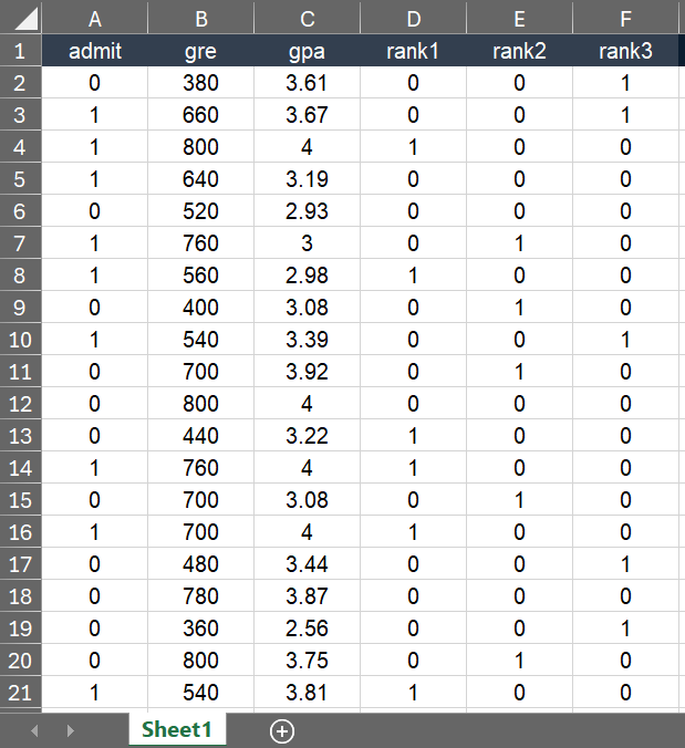
Suppose you are asked to perform logistic regression analysis in Excel to check whether a student will be admitted or not into graduate school based on their GRE and GPA grades along with the ranking of the undergraduate school they attended.
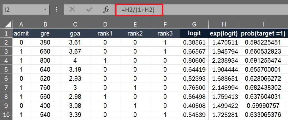
The raw data looks like the image shown below. We have 397 observations and 5 independent variables in our dataset. Data are in range A2:F398 in Excel. The column admit is a binary dependent variable in this case and the remaining columns contain data for independent variables.
Step 1 : Setting Initial Coefficients
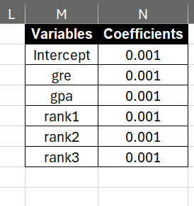
In this step, we are creating a coefficient table for independent variables and intercept. We are setting each coefficient to 0.001. Later we will be adjusting them to maximize the log likelihood.
- Enter intercept and independent variable names in range M2:M7.
- Enter initial values for coefficients as 0.001 in range N2:N7.
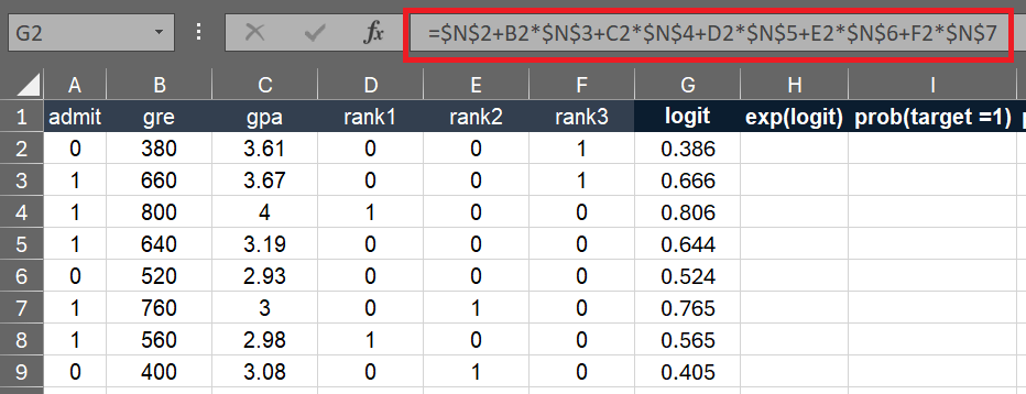
Step 2 : Calculations of Logistic Regression
It is linear combination of the independent variables weighted by their coefficients. To calculate logit, we need to multiply coefficients with values of independent variables and then sum them.
In Excel, enter the following formula in cell G2 and then paste it down to the last row i.e cell G398.
=$N$2+B2*$N$3+C2*$N$4+D2*$N$5+E2*$N$6+F2*$N$7
Alternative Method : If you have a lot of independent variables, it is inefficient to write out the lengthy formula above. Alternatively, you can use the SUMPRODUCT formula.
=$N$2+SUMPRODUCT(B2:F2,TRANSPOSE($N$3:$N$7))
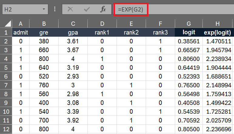
In this step, we simply take exponential value of the logit using the Excel's EXP() function. In cell H2, enter the following formula.
=EXP(G2)
The probability that the dependent variable y is 1 is calculated as:
prob(y=1) = exp(logit) / (1 + exp(logit))
In cell I2, enter the following formula and then paste it down to cell I398.
=H2/(1+H2)
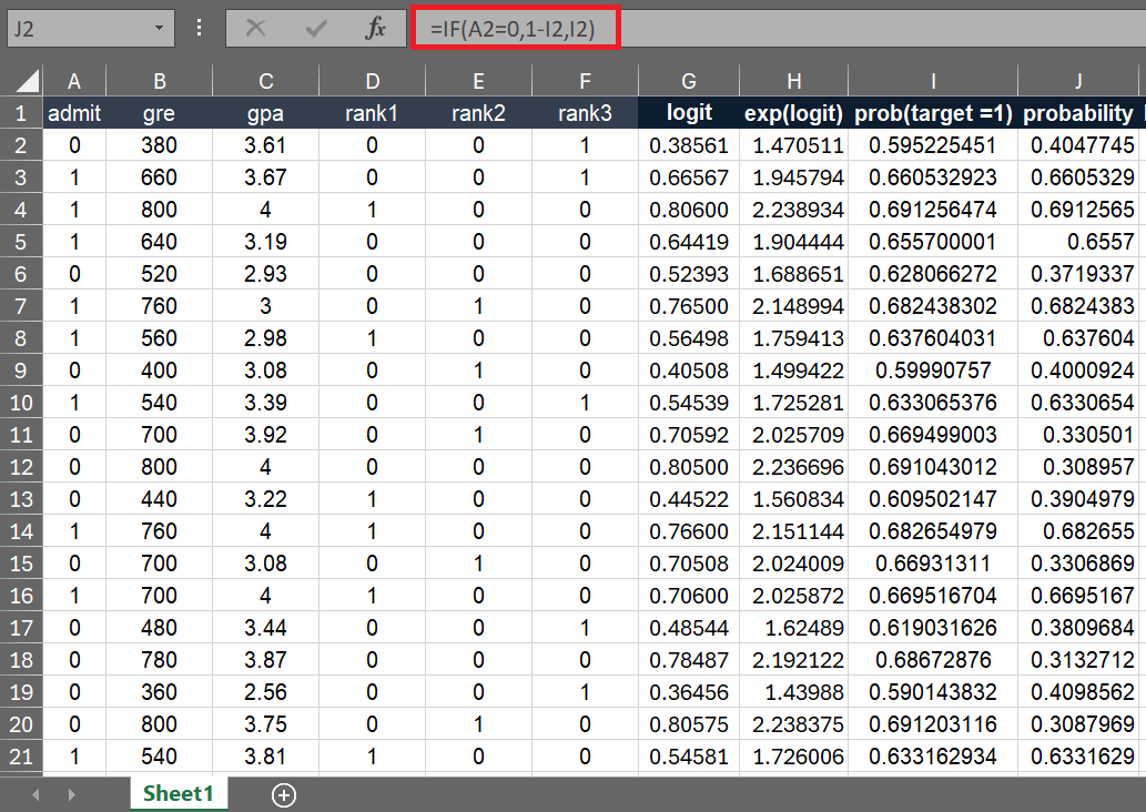
In this step, we are calculating the probability of the dependent variable (y) is either 0 or 1.
prob(y=0) = 1 - prob(y=1)
In cell J2, enter the following formula and then paste it down to cell J398.
=IF(A2=0,1-I2,I2)
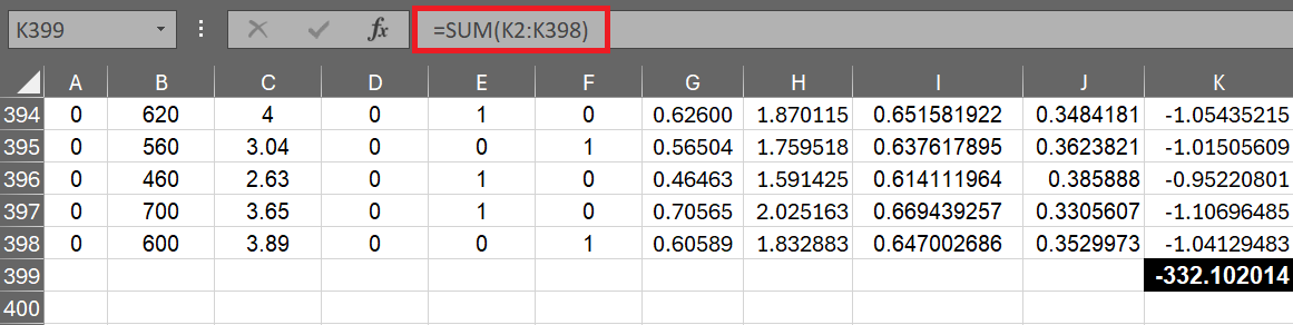
To calculate the log likelihood, we need to take the natural log of predicted probabilities.
In cell K2, enter the following formula to calculate the log likelihood and then paste it down to cell K398.
=LN(J2)

Next step is to sum the log likelihood for each observation. In the last row of the column i.e. cell K399, sum this column.
=SUM(K2:K398)
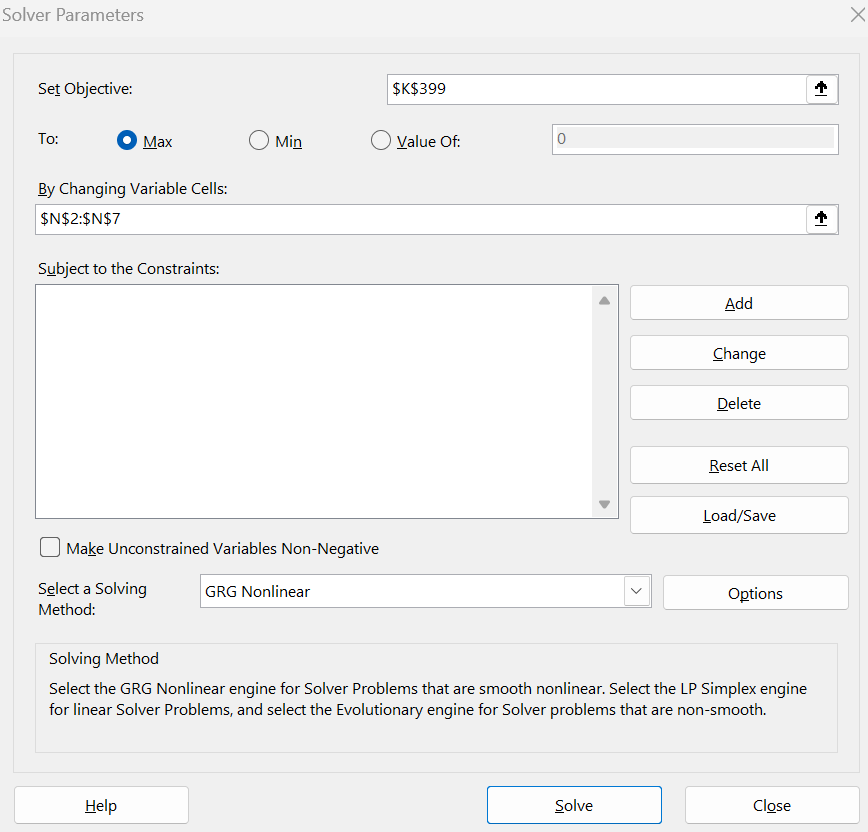
Step 3 : Maximizing Log Likelihood
In this step, we need to adjust the coefficients to maximize the log likelihood.
Excel's solver add-in will be used to optimizate the likelihood function.
After installing the solver add-in, follow the steps below.
- Go to the "Data" tab and click on "Solver".
- Set the objective function to the cell K399 containing the sum of the log-likelihood.
- Select "Max" in the "To:" section.
- By Changing Variable Cells: Select cells N2:N7 containing coefficients (including intercept).
- Make Unconstrained Variables Non-Negative: Uncheck this option.
- Choose the Solver engine GRG Nonlinear.
- Click "Solve" to run the optimization.
The final logistic regression coefficients and predicted probabilities are shown below.

Suppose you have a new data which was not used to build the logistic regression model. You need to estimate the predicted probability for the new data using the model you built in the previous steps.
| gre | gpa | rank1 | rank2 | rank3 |
|---|---|---|---|---|
| 650 | 3.67 | 0 | 0 | 1 |
All you need to do is drag the formula down (as shown in the previous steps) to the new data to calculate prob(y=1). Refer to the image below.

The standard error of a coefficient in logistic regression explains how reliable coefficient estimates are.

To calculate the standard error of coefficients, run the VBA code below.
Sub StandardErrors()
    Dim XData As String
    Dim MatrixSize As Long
    Dim CoeffData As String
    Dim outputStartingCell As String
    Dim i As Long, j As Long
    Dim Hessian() As Double
    Dim ws As Worksheet

    ' Set input values
    Set ws = ThisWorkbook.Sheets("Sheet1") ' Change sheet name if needed
    XData = "B2:F398"          ' Range for independent variables
    CoeffData = "N2:N7"       ' Range for coefficients (incld. intercept)
    outputStartingCell = "O2"  ' Starting cell where you want to populate standard errors (output)

    ' Initialize the Hessian matrix
    MatrixSize = Range(XData).Columns.Count + 1 ' Include intercept
    ReDim Hessian(1 To MatrixSize, 1 To MatrixSize)

    ' Read coefficient values from cells (adjust cell references as needed)
    Dim Coeff() As Double
    Dim rng As Range
    Set rng = ws.Range(CoeffData) ' Convert the string to a range
    ReDim Coeff(1 To rng.Cells.Count)
    i = 1
    For Each cell In rng
        Coeff(i) = cell.Value
        i = i + 1
    Next cell

    ' Read feature data from cells (adjust cell references as needed)
    Dim X() As Double
    Dim inputRange As Range
    Set inputRange = ws.Range(XData)
    n = inputRange.Rows.Count

    ReDim X(1 To n, 1 To MatrixSize)
    Dim rowIndex As Long, colIndex As Long
    For rowIndex = 1 To n
        X(rowIndex, 1) = 1 ' Intercept
        For colIndex = 1 To MatrixSize - 1
            X(rowIndex, colIndex + 1) = inputRange.Cells(rowIndex, colIndex).Value
        Next colIndex
    Next rowIndex

    ' Calculate the Hessian matrix
    Dim p_hat() As Double
    ReDim p_hat(1 To n)
    For rowIndex = 1 To n
        Dim Xb As Double
        Xb = 0
        For j = 1 To MatrixSize
            Xb = Xb + X(rowIndex, j) * Coeff(j)
        Next j
        p_hat(rowIndex) = Exp(Xb) / (1 + Exp(Xb)) ' Predicted probabilities
    Next rowIndex

    ' Calculate the Hessian elements
    For i = 1 To MatrixSize
        For j = 1 To MatrixSize
            Dim sum_term As Double
            sum_term = 0
            For rowIndex = 1 To n
                sum_term = sum_term + X(rowIndex, i) * X(rowIndex, j) * p_hat(rowIndex) * (1 - p_hat(rowIndex))
            Next rowIndex
            Hessian(i, j) = sum_term
        Next j
    Next i

    ' Invert the Hessian matrix
    Dim invHessian() As Double
    invHessian = InverseMatrix(Hessian)

    ' Calculate standard errors
    Dim se() As Double
    ReDim se(1 To MatrixSize)
    For i = 1 To MatrixSize
        se(i) = Sqr(invHessian(i, i))
    Next i

    ' Output standard errors to the worksheet
    ws.Range(outputStartingCell).Value = se(1) ' Intercept
    For i = 2 To MatrixSize
        ws.Range(outputStartingCell).Offset(i - 1, 0).Value = se(i)
    Next i

End Sub


Function InverseMatrix(mat() As Double) As Variant
    ' This function computes the inverse of a matrix using the Gaussian elimination method
    ' Note: This function assumes that the input matrix is square and invertible

    Dim n As Long
    n = UBound(mat, 1)

    Dim augmented() As Double
    ReDim augmented(1 To n, 1 To 2 * n)

    Dim i As Long, j As Long, k As Long
    Dim factor As Double

    ' Create augmented matrix [mat | I]
    For i = 1 To n
        For j = 1 To n
            augmented(i, j) = mat(i, j)
            augmented(i, j + n) = IIf(i = j, 1, 0)
        Next j
    Next i

    ' Perform Gaussian elimination
    For i = 1 To n
        ' Make the diagonal element 1
        factor = augmented(i, i)
        For j = 1 To 2 * n
            augmented(i, j) = augmented(i, j) / factor
        Next j

        ' Make the other elements in the column 0
        For k = 1 To n
            If k <> i Then
                factor = augmented(k, i)
                For j = 1 To 2 * n
                    augmented(k, j) = augmented(k, j) - factor * augmented(i, j)
                Next j
            End If
        Next k
    Next i

    ' Extract the inverse matrix
    Dim invMat() As Double
    ReDim invMat(1 To n, 1 To n)

    For i = 1 To n
        For j = 1 To n
            invMat(i, j) = augmented(i, j + n)
        Next j
    Next i

    InverseMatrix = invMat
End Function
- In Excel, open the VBA editor by pressing Alt + F11 keyboard shortcut key.
- Select Insert > Module to create a module.
- Paste the above macro code in the module.
- Close the VBA editor by clicking the 'X' in the top-right corner.
- Run the macro by pressing Alt + F8 and select "StandardErrors" macro
Set ws = ThisWorkbook.Sheets("Sheet1"): Change "Sheet1" to your desired sheet name.XData = "B2:F398": Specifies the range for independent variables. Modify "B2:F398" to match your data range.CoeffData = "N2:N7": Defines the range for coefficients including the intercept. Adjust "N2:N7" to the range for your coefficients.outputStartingCell = "O2": Sets the starting cell for outputting results. Change "O2" to the cell where you want to begin outputting data.
The z-statistic measures how many standard deviations a coefficient estimate is away from 0. A small p-value less than 0.05 means the coefficient of independent variable is significantly different from 0.
z-statistic = coefficient / standard error
To calculate z-statistic, enter the following formula in cell P2. Cell N2 contains coefficients and cell O2 contains standard error.
=N2 / O2
To calculate p-value, enter the following formula in cell Q2.
=2*(1-NORM.S.DIST(ABS(N2)/O2,1))
To calculate wald chi-square, all we need to do is to take square of z-statistics. In cell R2, enter the following formula.
=P2^2
The formula for calculating confidence intervals for a coefficient is as follows:
CI = coefficient ± z * Standard Error
Here z is the critical value. It is 1.96 for a 95% confidence interval
In cell S2, enter the following formula for lower confidence interval.
=N2 - 1.96*O2
In cell T2, enter the following formula for upper confidence interval.
=N2 + 1.96*O2
Standardized Coefficients help in understanding the relative importance of each independent variable. Variable with the largest absolute value of a standardized coefficient means the most important variable.
The formula for calculating confidence intervals for a coefficient is as follows:
Standardized Coefficient = (β * SDX) / (π / √3)
SDX is a standard deviation of an independent variable.
In cell U3, enter the following formula. Please note that it is not entered against intercept. Paste the formula down to the cells below to get standardized coefficients for each independent variable. In this formula, cell N3 refers to unstandardized coefficient; range B2:B398 refers to raw values of variable. By using the OFFSET function, this formula became dynamic and automatically changing the range of variables as it's pasted down.
=(N3*STDEV.S(OFFSET($B$2:$B$398,,ROW(A1)-1))/(PI()/SQRT(3)))
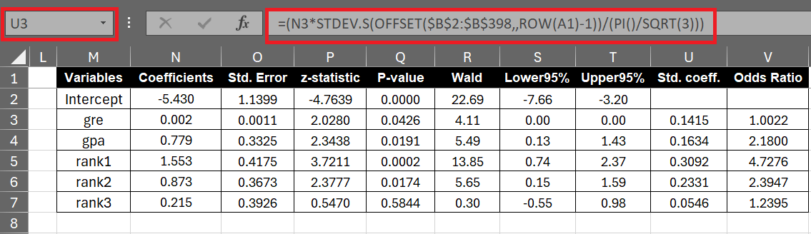
Odds ratio is exponential value of a coefficient. It means how the odds of the dependent variable change with each unit change in the independent variable.
In cell V3, enter the following formula to calculate odds ratio in Excel.
=EXP(N3)
The main model performance metrics of logistic regression are Area Under Curve (AUC) of the ROC Curve, AIC and Hosmer-Lemeshow (HL) Test.
AUC measures how well the model can differentiate between events (1) and non-events (0).
Insert the following VBA code by following the first four steps shown in this section of article.
Function AUROC(predictions As Range, actuals As Range) As Double
    Dim n As Long
    Dim tpr() As Double, fpr() As Double
    Dim sorted_indices() As Long
    Dim i As Long

    ' Check if the predictions and actuals ranges have the same number of elements
    If predictions.Count <> actuals.Count Then
        MsgBox "Predictions and actuals must have the same number of elements."
        AUROC = -1
        Exit Function
    End If

    n = predictions.Count
    ReDim tpr(0 To n + 1), fpr(0 To n + 1)

    ' Sort predictions and actuals in descending order of predictions
    sorted_indices = SortIndicesDescending(predictions)

    Dim num_pos As Long, num_neg As Long
    num_pos = WorksheetFunction.CountIf(actuals, 1)
    num_neg = n - num_pos

    If num_pos = 0 Or num_neg = 0 Then
        MsgBox "There must be both positive and negative actual values."
        AUROC = -1
        Exit Function
    End If

    Dim tp_count As Long, fp_count As Long
    tp_count = 0
    fp_count = 0

    ' Calculate TPR and FPR for each threshold
    For i = 1 To n
        If actuals.Cells(sorted_indices(i)).Value = 1 Then
            tp_count = tp_count + 1
        Else
            fp_count = fp_count + 1
        End If

        tpr(i) = tp_count / num_pos
        fpr(i) = fp_count / num_neg
    Next i

    ' Append (0,0) and (1,1) to the ROC curve
    tpr(0) = 0
    tpr(n + 1) = 1
    fpr(0) = 0
    fpr(n + 1) = 1

    ' Calculate AUC from the ROC curve using trapezoidal rule
    Dim auc As Double
    auc = 0
    For i = 1 To n
        auc = auc + (tpr(i) + tpr(i - 1)) * (fpr(i - 1) - fpr(i)) / 2
    Next i

    ' Ensure AUC is non-negative
    AUROC = Abs(auc)
End Function

Function SortIndicesDescending(predictions As Range) As Variant
    Dim i As Long, j As Long
    Dim temp As Double
    Dim indices() As Long
    Dim sorted_predictions() As Double

    Dim n As Long
    n = predictions.Count
    ReDim indices(1 To n)
    ReDim sorted_predictions(1 To n)

    For i = 1 To n
        indices(i) = i
        sorted_predictions(i) = predictions.Cells(i).Value
    Next i

    ' Simple bubble sort
    For i = 1 To n - 1
        For j = i + 1 To n
            If sorted_predictions(i) < sorted_predictions(j) Then
                ' Swap predictions
                temp = sorted_predictions(i)
                sorted_predictions(i) = sorted_predictions(j)
                sorted_predictions(j) = temp

                ' Swap indices
                temp = indices(i)
                indices(i) = indices(j)
                indices(j) = temp
            End If
        Next j
    Next i

    SortIndicesDescending = indices
End Function
After inserting the above code into the module, you can use the function =AUROC(prob(y=1),dependent variable) in any cell within your Excel workbook.
=AUROC(I2:I398,A2:A398)
AUC is used for model selection. Lower AIC values means better-fitting models. It penalizes models for their complexity and favors simpler models that explain the data well.
AIC = −2×log-likelihood+2×(Number of Independent Variables+1)
Cells K2:K398 refers to range of log-likelihood column. Cells B1:F1 refers to headers of independent variables.
=-2*SUM(K2:K398)+2*(COUNTA(B1:F1)+1)
A confusion matrix is used to evaluate the performance of a classification model. It compares the actual values with the model's predictions. You can refer to this tutorial - Confusion Matrix in Excel
The Hosmer-Lemeshow (HL) test is used to check the goodness of fit of a logistic regression model. It explains how well the predicted probabilities from the model match the actual outcomes.
Calculating Hosmer-Lemeshow (HL) Test in Excel

Deepanshu founded ListenData with a simple objective - Make analytics easy to understand and follow. He has over 10 years of experience in data science. During his tenure, he worked with global clients in various domains like Banking, Insurance, Private Equity, Telecom and HR.
Share Share Tweet