This tutorial explains how to create a ROC curve in MS Excel.
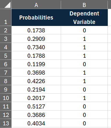
Please make sure that you have predicted probabilities and dependent variable columns in Excel as shown in the image below.
Step 1 : Calculate False Positive Rate and True Positive Rate
The following VBA code calculates False Positive Rate (FPR) and True Positive Rate (TPR) for each predicted probability values, along with Area Under Curve (AUC) in Excel.
Sub ROC()

    Dim n As Long
    Dim tpr() As Double, fpr() As Double
    Dim sorted_indices() As Long
    Dim i As Long
    Dim predictions As Range, actuals As Range, startCell As Range

    ' Prompt user to select the range for predictions
    On Error Resume Next
    Set predictions = Application.InputBox("Select the range for predicted probabilties:", Type:=8)
    On Error GoTo 0

    ' Check if the user canceled the input box
    If predictions Is Nothing Then
        MsgBox "You canceled the selection for predictions range."
        Exit Sub
    End If

    ' Prompt user to select the range for actuals
    On Error Resume Next
    Set actuals = Application.InputBox("Select the range for dependent variable:", Type:=8)
    On Error GoTo 0

    ' Check if the user canceled the input box
    If actuals Is Nothing Then
        MsgBox "You canceled the selection for actuals range."
        Exit Sub
    End If

    ' Check if the predictions and actuals ranges have the same number of elements
    If predictions.Count <> actuals.Count Then
        MsgBox "Predictions and actuals must have the same number of elements."
        AUC = -1
        Exit Sub
    End If

    n = predictions.Count
    ReDim tpr(0 To n + 1), fpr(0 To n + 1)

    ' Sort predictions and actuals in descending order of predictions
    sorted_indices = SortIndicesDescending(predictions)

    Dim num_pos As Long, num_neg As Long
    num_pos = WorksheetFunction.CountIf(actuals, 1)
    num_neg = n - num_pos

    If num_pos = 0 Or num_neg = 0 Then
        MsgBox "There must be both positive and negative actual values."
        AUC = -1
        Exit Sub
    End If

    Dim tp_count As Long, fp_count As Long
    tp_count = 0
    fp_count = 0

    ' Calculate TPR and FPR for each threshold
    For i = 1 To n
        If actuals.Cells(sorted_indices(i)).Value = 1 Then
            tp_count = tp_count + 1
        Else
            fp_count = fp_count + 1
        End If

        tpr(i) = tp_count / num_pos
        fpr(i) = fp_count / num_neg
    Next i

    ' Append (0,0) and (1,1) to the ROC curve
    tpr(0) = 0
    tpr(n + 1) = 1
    fpr(0) = 0
    fpr(n + 1) = 1


    ' Prompt user to select the starting cell for output
    On Error Resume Next
    Set startCell = Application.InputBox("Select the cell where output should begin:", Type:=8)
    On Error GoTo 0

    ' Check if the user canceled the input box
    If startCell Is Nothing Then
        MsgBox "You canceled the selection for starting cell."
        Exit Sub
    End If

    ' Output tpr array to cells
        startCell.Offset(0, 0).Value = "FPR"
        startCell.Offset(0, 1).Value = "TPR"
        startCell.Offset(0, 2).Value = "AUC"

    For i = LBound(tpr) To UBound(tpr)
        startCell.Offset(i + 1, 0).Value = fpr(i)
        startCell.Offset(i + 1, 1).Value = tpr(i)
    Next i

    'Calculate AUC from the ROC curve using trapezoidal rule
    Dim AUC2 As Double
    AUC2 = 0
    For i = 1 To n
        AUC2 = AUC2 + (tpr(i) + tpr(i - 1)) * (fpr(i - 1) - fpr(i)) / 2
    Next i

    ' Ensure AUC is non-negative
    AUC = Abs(AUC2)
    startCell.Offset(1, 2).Value = AUC

End Sub

Function SortIndicesDescending(predictions As Range) As Variant
    Dim i As Long, j As Long
    Dim temp As Double
    Dim indices() As Long
    Dim sorted_predictions() As Double

    Dim n As Long
    n = predictions.Count
    ReDim indices(1 To n)
    ReDim sorted_predictions(1 To n)

    For i = 1 To n
        indices(i) = i
        sorted_predictions(i) = predictions.Cells(i).Value
    Next i

    ' Simple bubble sort
    For i = 1 To n - 1
        For j = i + 1 To n
            If sorted_predictions(i) < sorted_predictions(j) Then
                ' Swap predictions
                temp = sorted_predictions(i)
                sorted_predictions(i) = sorted_predictions(j)
                sorted_predictions(j) = temp

                ' Swap indices
                temp = indices(i)
                indices(i) = indices(j)
                indices(j) = temp
            End If
        Next j
    Next i

    SortIndicesDescending = indices
End Function
- In Excel, open the VBA editor by pressing Alt + F11 keyboard shortcut key.
- Select Insert > Module to create a module.
- Paste the above VBA code in the module.
- Close the VBA editor by clicking the 'X' in the top-right corner.
- Run the macro by pressing Alt + F8 and select "ROC" macro
- This macro asks you to select the range for predicted probabilities and binary dependent variable (excluding headers).
- Then choose a cell where output table containing FPR and TPR values should start.
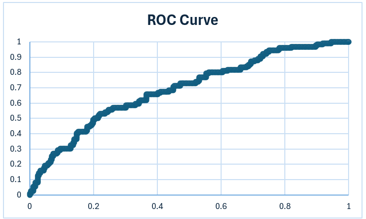
Step 2 : Create Scatter Chart for ROC Curve
Next step is to create a ROC Curve by following the steps below :
- Select range for false positive rate and true positive rate. In this case, it is D3:E401.
- Go to Insert tab in the ribbon and then click on Scatter(X, Y) chart type.
- Right-click on the X-axis and then Select Format Axis from the menu.
- Set the Maximum bound to 1 under the Bounds section.
- Right-click on the Y-axis and then Select Format Axis from the menu.
- Set the Maximum bound to 1 under the Bounds section.
How to Calculate AUC
The Trapezoidal Rule is used to find the area under the curve using the false positive rate and true positive rate at different cutoffs.
( fpri+1 – fpri ) * ( tpri + tpri+1 ) / 2
Let's say you have values for false positive rate in cells D3:D401 and values for true positive rate in cells E3:E401.
In cell G4, enter the following formula :
=(D4-D3)*(E4+E3)
Then paste the formula above till the cell just before the last row (up to cell G400). Please note that we need to ignore the last cell where both TPR and FPR are 1.
To calculate AUC, use this formula =SUM(G4:G400)/2.
How to Calculate Confusion Matrix in Excel
Excel Template : Gain and Lift Charts
How to Build Logistic Regression in Excel
Free Excel Add-In for Logistic Regression

Deepanshu founded ListenData with a simple objective - Make analytics easy to understand and follow. He has over 10 years of experience in data science. During his tenure, he worked with global clients in various domains like Banking, Insurance, Private Equity, Telecom and HR.
Share Share Tweet