This tutorial explains how to explore data with PROC UNIVARIATE. It is one of the most powerful SAS procedure for running descriptive statistics as well as checking important assumptions of various statistical techniques such as normality, detecting outliers.
PROC UNIVARIATE has powerful features but is less popular than PROC MEANS. Many SAS analysts use PROC MEANS for basic statistics. However, PROC UNIVARIATE offers more options.
See the main difference between these two SAS procedures.
- PROC MEANS can calculate various percentile points such as 1st, 5th, 10th, 25th, 50th, 75th, 90th, 95th, 99th percentiles but it cannot calculate custom percentiles such as 20th, 80th, 97.5th, 99.5th percentiles. Whereas, PROC UNIVARIATE can run custom percentiles.
- PROC UNIVARIATE can calculate extreme observations - the five lowest and five highest values. Whereas, PROC MEANS can only calculate MAX value.
- PROC UNIVARIATE supports normality tests to check normal distribution. Whereas, PROC MEANS does not support normality tests.
- PROC UNIVARIATE generates multiple plots such as histogram, box-plot, steam leaf diagrams whereas PROC MEANS does not support graphics.
In the example below, we would use sashelp.shoes dataset. SALES is the numeric (or measured) variable.
proc univariate data = sashelp.shoes;
var sales;
run;
1. Moments : Count, Mean, Standard Deviation, SUM etc
2. Basic Statistics : Mean, Median, Mode etc
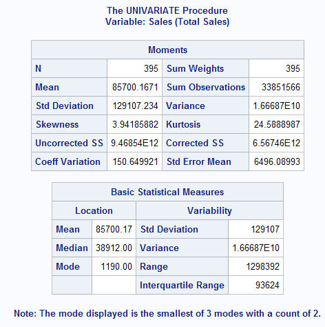
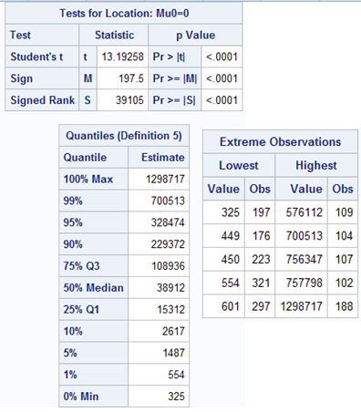
3. Tests for Location : one-sample t-test, Signed Rank test.
4. Percentiles (Quantiles)
5. Extreme Observations - first smallest and largest values against their row position.
Suppose you are asked to calculate basic statistics of sales by region. In this case, region is a grouping (or categorical) variable. The CLASS statement is used to define categorical variable.
proc univariate data = sashelp.shoes;
var sales;
class region;
run;
See the output shown below -
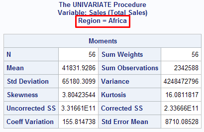
The similar output was generated for other regions - Asia, Canada, Eastern Europe, Middle East etc.
Suppose you want only percentiles to be appeared in output window. By default, PROC UNIVARIATE creates five output tables : Moments, BasicMeasures, TestsForLocation, Quantiles, and ExtremeObs. The ODS SELECT can be used to select only one of the table. The Quantiles is the standard table name of PROC UNIVARIATE for percentiles which we want. ODS stands for Output Delivery System.
ods select Quantiles;
proc univariate data = sashelp.shoes;
var sales;
class region;
run;
The ODS TRACE ON produces name and label of tables that SAS Procedures generates in the log window.
ods trace on;
proc univariate data = sashelp.shoes;
var sales;
run;
ods trace off;
The ODS OUTPUT statement is used to write output in results window to a SAS dataset. In the code below, temp would be the name of the dataset in which all the percentile information exists.
ods output Quantiles = temp;
proc univariate data = sashelp.shoes;
var sales;
class region;
run;
ods output close;
Like we generated percentiles in the previous example, we can generate extreme values with extremeobs option. The ODS OUTPUT tells SAS to write the extreme values information to a dataset named outlier. The "extremeobs" is the standard table name of PROC UNIVARIATE for extreme values.
ods output extremeobs = outlier;
proc univariate data = sashelp.shoes;
var sales;
class region;
run;
ods output close;
Most of the statistical techniques assumes data should be normally distributed. It is important to check this assumption before running a model.
There are multiple ways to check Normality :
- Plot Histogram and see the distribution
- Calculate Skewness
- Normality Tests
Histogram shows visually whether data is normally distributed.
proc univariate data=sashelp.shoes NOPRINT;
var sales;
HISTOGRAM / NORMAL (COLOR=RED);
run;
It also helps to check whether there is an outlier or not.
Skewness is a measure of the degree of asymmetry of a distribution. If skewness is close to 0, it means data is normal.
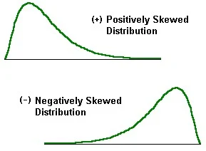
A positive skewed data means that there are a few extreme large values which turns its mean to skew positively. It is also called right skewed.
Positive Skewness : If skewness > 0, data is positively skewed. Another way to see positive skewness : Mean is greater than median and median is greater than mode.
A negative skewed data means that there are a few extreme small values which turns its mean to skew negatively. It is also called left skewed.
Negative Skewness : If skewness < 0, data is negatively skewed. Another way to see negative skewness : Mean is less than median and median is less than mode.
- If skewness < −1 or > +1, the distribution is highly skewed.
- If skewness is between −1 and −0.5 or between 0.5 and +1, the distribution is moderately skewed.
- If skewness > −0.5 and < 0.5, the distribution is approximately symmetric or normal.
ods select Moments;
proc univariate data = sashelp.shoes;
var sales;
run;
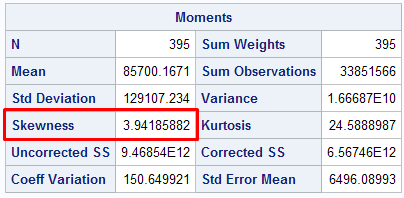
Since Skewness is greater than 1, it means data is highly skewed and non-normal.
The NORMAL keyword tells SAS to generate normality tests.
ods select TestsforNormality;
proc univariate data = sashelp.shoes normal;
var sales;
run;
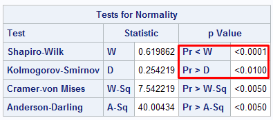
The two main tests for normality are as follows :
It states that the null hypothesis - distribution is normal.
In the example above, p value is less that 0.05 so we reject the null hypothesis. It implies distribution is not normal. If p-value > 0.05, it implies distribution is normal.
This test performs well in small sample size up to 2000.
In this test, the null hypothesis states the data is normally distributed.
If p-value > 0.05, data is normal. In the example above, p-value is less than 0.05, it means data is not normal.
This test can handle larger sample size greater than 2000.
With PCTLPTS= option, we can calculate custom percentiles. Suppose you need to generate 10, 20, 30, 40, 50, 60, 70, 80, 90, 100 percentiles.
proc univariate data = sashelp.shoes noprint;
var sales;
output out = temp
pctlpts = 10 to 100 by 10 pctlpre = p_;
run;
The OUTPUT OUT= statement is used to tell SAS to save the percentile information in TEMP dataset. The PCTLPRE= is used to add prefix in the variable names for the variable that contains the PCTLPTS= percentile.
Suppose you want to calculate 97.5 and 99.5 percentiles.
proc univariate data = sashelp.shoes noprint;
var sales;
output out = temp
pctlpts = 97.5,99.5 pctlpre = p_;
run;
The Winsorized and Trimmed Means are insensitive to Outliers. They should be reported rather than mean when the data is highly skewed.
Trimmed Mean : Removing extreme values and then calculate mean after filtering out the extreme values. 10% Trimmed Mean means calculating 10th and 90th percentile values and removing values above these percentile values.
Winsorized Mean : Capping extreme values and then calculate mean after capping extreme values at kth percentile level. It is same as trimmed mean except removing the extreme values, we are capping at kth percentile level.
In the example below, we are calculating 20% Winsorized Mean.
ods select winsorizedmeans;
ods output winsorizedmeans=means;
proc univariate winsorized = 0.2 data=sashelp.shoes;
var sales;
run;

Percent Winsorized in Tail : 20% of values winsorized from each tail (upper and lower side)
Number Winsorized in Tail : 79 values winsorized from each tail
In the example below, we are calculating 20% trimmed Mean.
ods select trimmedmeans;
ods output trimmedmeans=means;
proc univariate trimmed = 0.2 data=sashelp.shoes;
var sales;
run;
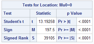
It tests the null hypothesis that mean of the variable is equal to 0. The alternative hypothesis is that mean is not equal to 0. When you run PROC UNIVARIATE, it defaults generates sample t-test in 'Tests for Location' section of output.
ods select TestsForLocation;
proc univariate data=sashelp.shoes;
var sales;
run;
Since p-value is less than 0.05, we reject the null hypothesis. It concludes the mean value of the variable is significantly different from zero.
PROC UNIVARIATE generates the following plots :
- Histogram
- Box Plot
- Normal Probability Plot
The PLOT keyword is used to generate plots.
proc univariate data=sashelp.shoes PLOT;
var sales;
run;


Very good article. I am just loving listendata.
ReplyDeleteThank you for your appreciation. Cheers!
DeleteNevermind, I skipped the part. Thank you so much. I will bookmark your page. You are the best
ReplyDeleteThe way you described the article, really appreciated..!!
ReplyDeleteim completed base sas course now im looking for job if any job vaccany for fresher
DeleteThis is really nice platform to learn SAS
ReplyDeleteGreat tutoring Mr Bhalla.... I always look for your material on a particular topic I am searching for.Please keep posting. Can you make a series on PROC SGPLOTS please.... Thank you.
ReplyDeleteGreat brother
ReplyDeleteWhen everyone around the world is busy minting money to teach. You are doing a great job by providing valuable information for free. your explanation is so easy to understand and also almost cover all the area.
ReplyDeleteGreat job. Keep up the good work.
Can i get normality test results in output dataset using proc univariate
ReplyDeleteI am big fan of your work. God bless you.
ReplyDeleteCould you pls advise me the syntax how to import data from PDF file to sas. Thanks in advance!
ReplyDeleteNice explanations Deepanshu. Very clear explanation.
ReplyDelete